As a spatial data specialist, one of my contributions to The Common Line project has been to help devise the way in which members of the public will locate, navigate to, and interact with individual points along it. The philosophy for the project is to remain as ‘open source’ as possible, so this means avoiding google or other propriety web services, which in many ways adds to the challenge, but ultimately gives us more flexibility and control.
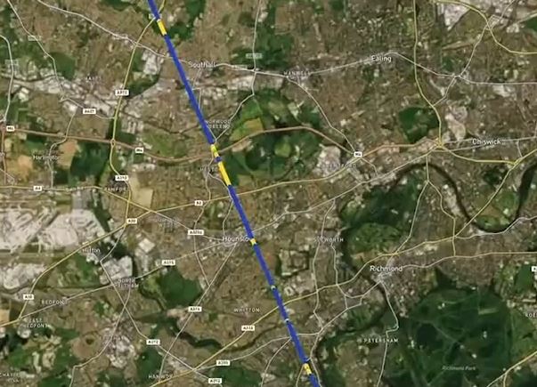
There are various elements that require consideration in realising our vision of The Common Line, in which individuals and small groups will want to interact with and share their experiences and perceptions of the world around them. The first element is how participants will visualise and locate the line to identify a particular point of interest they would like to visit. This may be the nearest point to their house or place of work, or perhaps a point that is located in an area that the participant wishes to explore/visit. Geographical Information Systems (GIS) analysis was used to determine the longest continuous line across Great Britain that does not cross any tidally-influenced stretches of Water. In practice, this meant bounding the line by the tidal limits of the Rivers Thames and the Border Esk in England, and the River Forth in Scotland. Once the line was determined, we needed to decide on an appropriate spacing of tree-planting locations along the line. After consultation with forestry experts, 20 m was agreed on as an appropriate spacing for the line to be considered a linear forest. The Common Line is over 880 km in length, and with points spaced every 20 m along it, there are more than 44 000 unique locations to consider!
Next we needed a way to ‘classify’ each point to identify which are suitable for planting real and virtual trees, and perhaps even to say something about what species would be best suited for the specific location. From the outset, we knew the procedure for reaching an accurate classification for the points would be an iterative process. Given the scale of the task, an automated approach is required for the first iteration, with project-team validation and correction applied in subsequent iterations – firstly using satellite imagery and Ordnance Survey data for urban areas, and secondly using ‘in situ’ observations uploaded by members of The Common Line community.
For this preliminary automated classification, we decided to use the NERC Centre for Ecology and Hydrology Land Cover Map 2015 (LCM2015). This data product uses multispectral satellite observations to divide the whole of the UK land surface into 25 m by 25 m squares, and identifies each square as 1 of 21 land-cover classes. Using GIS analysis, we extract the LCM2015 class for every point on the common line – table 1 shows a summary of this analysis.
| LCM2015 class | Description of habitat | No. points on TCL | % |
| 1 | Broadleaf Woodland | 3048 | 6.9 |
| 2 | Coniferous woodland | 3174 | 7.2 |
| 3 | Arable & Horticulture | 4329 | 9.8 |
| 4 | Improved grassland | 12376 | 28.1 |
| 5 | Neutral grassland | 78 | 0.2 |
| 6 | Calcareous grassland | 189 | 0.4 |
| 7 | Acid grassland | 6957 | 15.8 |
| 9 | Heather | 1981 | 4.5 |
| 10 | Heather grassland | 4224 | 9.6 |
| 11 | bog | 1390 | 3.2 |
| 12 | Inland rock | 525 | 1.2 |
| 14 | Freshwater | 1040 | 2.4 |
| 17 | Littoral rock | 5 | 0.01 |
| 20 | Urban | 1124 | 2.6 |
| 21 | Suburban | 3530 | 8.0 |
Whilst interesting to see how many points are located in the different landcover areas, we really need the classification to be useful for the community to help them determine how they want to interact with the points on the line. For instance, we need the system to provide information on which points have already been planted – either real or virtual trees; which locations could be planted in the future; and which are not suitable or not accessible. To this end, we came up with a simpler classification system for points on the common Line (table 2), which is a sort of ‘conversion table’ based initially on the LCM2015 classes, but eventually to be validated on the ground by ‘tree scouts’. In the current pilot study, we use an even simpler classification system of (i) Existing Trees (green), (ii) Plantable areas (orange), (iii) Unsuitable areas (red) and (iv) inaccessible areas (blue). The preliminary results can be seen on the online viewer here.
| Target class | Description | A priori LCM 2015 Classes | |
| 1 | Existing trees | Pre-existing woodland. Potential for ‘assimilating’ existing trees into TCL | 1, 2 |
| 2 | Plantable | Suitable habitat. Permissions and access pending. | 3, 4, 5, 6, 7 |
| 3 | Unsuitable | Habitat unsuitable for trees | (9, 10), 11, 12, 14, 17 |
| 4 | Inaccessible | Suitable habitat but access problematic (TBD in next iteration of classification) | 20, 21 |
| 5 | Unknown | Requires insitu inspection to determine suitability (by a ‘Tree Scout’ ?) | TBD following next classification
|
If you explore the satellite-LCM layer of the viewer, you may notice some points are potentially being misclassified (e.g. in parts of the Scottish Highlands). In interpreting how the points have been classified, it is necessary to understand that in this early-stage iteration, all we have included is information about 1 ‘snapshot’ in time of the spectral properties (colour) of UK land cover, so there is not yet any information about permissions/access. What is clear, is that one of the future iterations needs to include a process for designating areas where access is a problem (e.g. airports), despite them being theoretically plantable based on the spectral properties.
There are several other reasons why these points need in situ validation, such as recent changes in land-use which would mean that the 2015 satellite data used to derive the LCM2015 is now out of date. It is also worth remembering that the process for deriving the classifications from the satellite data can never be 100% accurate, in particular where there are variations in spectral properties at the sub-grid scale (variations in shorter scales than 25 m). Finally, the fact that the LCM2015 is a ‘raster’ dataset (i.e. treats the land surface as a regular grid of square cells) means that ‘edge effects’ exist at the boundaries of differing landcover types. In these locations, points are likely to be misclassified due to there being ‘mixed pixels’, so one of the iteration steps may require us (or community volunteers?) to look at each boundary between landcover types and manually check these are being correctly classified.
While we have added a ‘touch of class’ to the project, there is clearly much more to do before we reach the point of having an operational database of tree-planting locations on the line – watch this space!
Dr Steven Palmer – August 2018